1 #!/usr/bin/env python
   2 # v0.26a 21 July 2014 author: Brian Fiedler
   3 # for data and confirming plots see:
   4 # http://www.cawcr.gov.au/projects/verification/POP3/POP3.html
   5 from __future__ import print_function #allows this program to still work with python2
   6 from pylab import *
   7 
   8 filename="POP_3cat_2003.txt" #available from above site
   9 dotmult = 4 # for scaling dot size in reliability diagram
  10 dpi=98 # smaller value makes smaller plot
  11 
  12 print("attempt to read",filename)
  13 lines=open(filename).readlines()
  14 
  15 # verif will be a dictionary, with  keys as percents: 0, 10, 20 ... 100
  16 # keys will retrieve a list of binary events (1's and 0's) on days forecast for that PoP
  17 verif = {} #initialize empty dictionary
  18 for p in range(0,105,10): # keys will be percents: 0, 10, 20...100
  19     verif[p]=[] # initialize empty list, will be populated as list of 1's and 0's 
  20 nt=0 # total number of days in dataset with non-missing forecast and obs
  21 nr=0 # total number of days in dataset with rain 
  22 # note in the following, daily rain amount < 0.3 mm is not considered a rain event
  23 for line in lines[1:]: #skip header line
  24     v = line.split() # split line at white space
  25     mm=float(v[3]) # observed daily rainfall
  26     p1=float(v[5]) # forecast probability for 0.3<= mm <= 4.4
  27     p2=float(v[6]) # forecast probability for mm >= 4.5
  28     if p1<0 or p2<0 or mm>998.: continue # missing forecast or missing data 
  29     prob=round(100*(p1+p2)) # probability of precip ( meaning rain >= 0.3mm) 
  30     rained = ( mm >= 0.3 )*1 # 1 means rain observed on day, 0 no rain 
  31     nt += 1  # increment total days
  32     nr += rained # increment rain days
  33     verif[prob].append(rained)  # append to the list of 1's and 0's
  34 climo=1.*nr/nt  # assume that the dataset average is also the climatology
  35 print("\nclimo,frequency of days with rain events:", climo)
  36 
  37 # Make the reliability diagram, and compute Brier scores
  38 bs=0. # will be Brier score 
  39 bsref=0. # will be Brier score using climo for forecast
  40 n=0 # will be number of events in Brier calculation; should be n==nt
  41 reli=0. # reliability, for Brier decomposition
  42 reso=0. # resolution, for Brier decomposition
  43 freqs=[] # freq of rain observed for that percent prediction
  44 nobs=[] # number of obs (for size of dot in reliability diagram)
  45 colors=[] # red dots will be denote skill, blue dots denote no skill
  46 pops=[] # list of PoP, as decimal (0., .1, ... 1.)
  47 print("\nPoP      observed freq     number of forecasts")
  48 for k in sorted(verif.keys()):
  49     pop=k/100. # convert percent to a probability
  50     q=verif[k] # list of 1's and 0's, from days with the forecasted pop
  51     lq=len(q) # number of obs
  52     ra=sum(q) # number of 1's
  53     if lq==0: continue # skip if no days were forecast for this PoP
  54     pops.append(pop) # store to use as x coord in plot 
  55     freq= float(ra) / lq # frequency of occurence
  56     print(pop, freq, lq )
  57     freqs.append(freq) # for y coord
  58     nobs.append(lq) # for dot size
  59     if abs(freq-climo) < abs(freq-pop): #for dot color
  60         colors.append('b') # blue means no skill
  61     else:
  62         colors.append('r') # red means skill
  63     reli += lq*(pop-freq)**2  # increment reliability 
  64     reso += lq*(freq-climo)**2 # increment resolution
  65     for event in q:
  66         bs += (pop-event)**2
  67         bsref += (climo-event)**2
  68         n+=1
  69 if nt!=n: print("should be equal:",n,nt)
  70 bs = bs/nt # divide sum of squares by number of squares
  71 bsref = bsref/nt
  72 print("\nBrier Score:",bs)
  73 print("Brier climo reference score:",bsref)
  74 bss = 1. - bs/bsref
  75 print("Brier skill score:",bss)
  76 # compute Brier decompostion
  77 unc=climo*(1-climo) # the uncertainty
  78 reli = reli/nt # reliability
  79 reso = reso/nt # resolution
  80 print("reli:",reli)
  81 print("reso:",reso)
  82 print("unc:",unc)
  83 bs2 = reli-reso+unc # alternative way to calculate Brier score
  84 print("Brier as reli-reso+unc:",bs2)
  85 print("  should be close to zero bs2-bs:",bs2-bs) # check the bs2 = bs
  86 
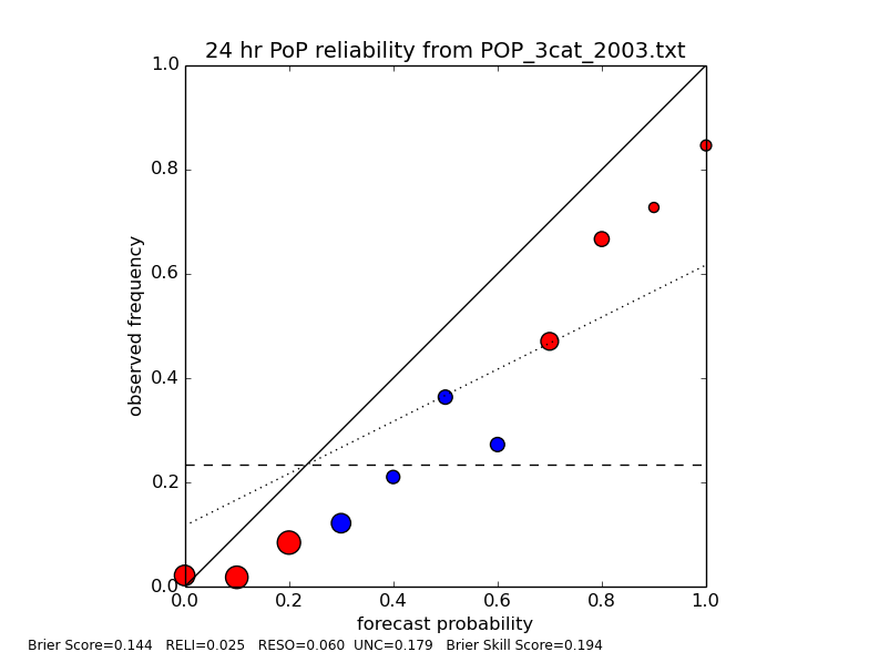
  87 # Plot the reliability diagram
  88 #print(freqs,obs,nobs,colors)
  89 caption_form="Brier Score={0:5.3f}   RELI={1:5.3f}   RESO={2:5.3f}  UNC={3:5.3f}   Brier Skill Score={4:5.3f}"
  90 caption_string=caption_form.format(bs,reli,reso,unc,bss)
  91 print(caption_string)
  92 dotsize=[dotmult*x for x in nobs] # make dot area proportional to number of obs 
  93 scatter(pops,freqs,s=dotsize,c=colors,clip_on=False)
  94 plot([0.,1.],[climo,climo],'k--') # climatology forecast
  95 plot([0.,1.],[0,1],'k-') # probability forecast
  96 plot([0.,1.],[climo/2., (1+climo)/2.],'k:') # no skill line
  97 axes().set_aspect('equal')
  98 axes().set_xlim([0,1]) # note xlim([0,1]) also works
  99 axes().set_ylim([0,1])
 100 title('24 hr PoP reliability from '+filename)
 101 ylabel('observed frequency')
 102 xlabel('forecast probability')
 103 text( -.3, -.12, caption_string, fontsize=9, transform=axes().transAxes) # http://wiki.scipy.org/Cookbook/Matplotlib/Transformations
 104 #show()
 105 savefig('reliability.png',dpi=dpi)
 106 clf() # clear the figure
 107 
 108 
 109 # computations for ROC plot  and Relative Value plot
 110 thresholds=[] # initialize empty lists
 111 hitrates=[]
 112 farates=[]
 113 ks = sorted(verif.keys()) # all the PoP percents
 114 cls=[n/100. for n in range(1,100) ] # C/L's for relative value curves
 115 rvs=[] # will be list of lists, each list defines a curve for a given C/L
 116 # from Wilks Fig 7.1: a=hits   b=false positives c=misses  d=true negatives
 117 #for k in [-5.01]+ks[:-1]+[100.0001]: # ignore last key, it cannot be a threshold
 118 for k in [-5.1]+ks[:] : # -5.1 makes the first threshold=-.001
 119     a = 0
 120     b = 0
 121     c = 0
 122     d = 0
 123     n = 0
 124 # thresholds will be stored as decimal for plot labels. thresholds halfway between keys
 125     threshold=k/100.+.05 #  .05 is arbitrary ... could be .01 - .09
 126     if threshold>1.: threshold=1.001 # looks nicer in ROC label
 127     thresholds.append(threshold) #used only for labels
 128     for m in ks:
 129         q=verif[m] # list of 1s and 0s
 130         lq=len(q) # number of events
 131         sq=sum(q) # number of positive events (1s) 
 132         n += lq
 133         if m<=k: # the PoP is less than the threshold, forecast no rain
 134             c += sq # misses
 135             d += lq - sq # true negatives
 136         else: # the PoP is above the threshold, forecast rain
 137             a += sq # hits
 138             b += lq - sq # false detections
 139 # Wilks page 324, Value Score
 140 # EE means expected expense
 141 # C is cost (in dollars)
 142 # L is loss (in dollars)
 143 # EE_perfect= C*climo 
 144 # if cl<=climo, take action on all days: EE_clim = C 
 145 # if cl>=climo, do nothing based on climo: EE_clim = L*climo 
 146 # EE_forecast: C*a + C*b - L *c
 147 # vs = (EE_forecast - EE_clim)/(EE_perfect - EE_clim)
 148 # In the following, all terms are divided by L, so you see ratio cl=C/L
 149     rv=[] # will be a list of value score, for the threshold
 150     n=float(n) # needed for python2, otherwise integer divide yields 0
 151     for cl in cls:
 152         if cl<climo:
 153             vs = ( cl*( a/n + b/n) + c/n  -cl )/( cl*climo - cl )
 154         else:
 155             vs = ( cl*( a/n + b/n) + c/n - climo )/( cl*climo - climo)
 156         rv.append(vs)
 157     rvs.append(rv) # append completed list         
 158     hitrates.append( float(a)/(a+c) )
 159 # see Wilks 7.11 and 7.13 for distinction between FA rate and ratio!!
 160 #    farates.append( float(b)/(a+b) ) # false alarm RATIO, not correct for RoC
 161     farates.append( float(b)/(d+b) ) # false alarm RATE,  correct for RoC curve
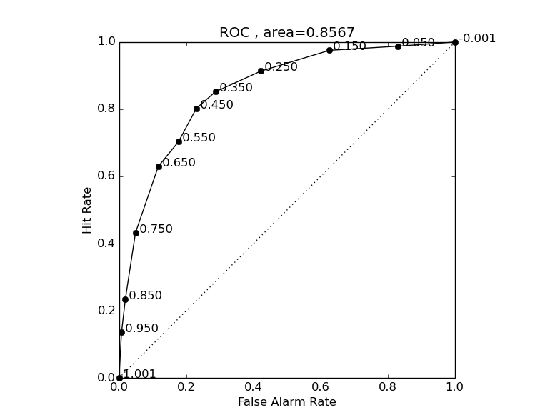
 162 area=0. # initialize computation of area under ROC curve
 163 for n in range( len(hitrates) -1 ):
 164     area += -.5*(hitrates[n+1]+hitrates[n])*(farates[n+1]-farates[n])
 165 areaf= "%5.4f" % area # will be included in plot title
 166 #print(farates,hitrates)
 167 
 168 # plot ROC curve
 169 plot(farates,hitrates,'ok-',clip_on=False)
 170 plot([0.,1.],[0,1],'k:')
 171 title('ROC , area='+areaf)
 172 xlabel('False Alarm Rate')
 173 ylabel('Hit Rate')
 174 axes().set_aspect('equal') # square plot
 175 axes().set_xlim([0,1])
 176 axes().set_ylim([0,1])
 177 i=0
 178 for x,y in zip(farates,hitrates):
 179     thresh = ' %5.3f' % thresholds[i]
 180     text(x,y,thresh,fontsize=12) # label each point in ROC with threshold
 181     i+=1
 182 savefig('ROC.png',dpi=dpi)
 183 clf()
 184 #print(rva)
 185 
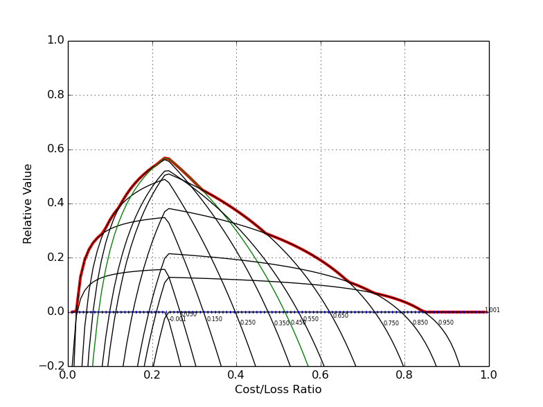
 186 # plot relative value curves
 187 rvmax=[] # list for envelope curve
 188 for i in range(len(rvs[0])): # cycle through each C/L
 189     rvmax.append( max([ rv[i]  for rv in rvs]) ) # max at the C/L
 190 m=0
 191 print("\nRelative value curves")
 192 for rv in rvs: # plot relative value curve for each threshold
 193     print("m=",m,"   threshold=",thresholds[m],"  max rv=",max(rv))
 194     if m==5:
 195         plot(cls,rv,'g-') # green for threshold=.45 is of interest here
 196     else:
 197         plot(cls,rv,'k-')
 198     xy=list(zip(cls,rv)) #prepare to make labels
 199     xy.reverse() # (x,y) coordinates are now from right to left
 200     for x,y in xy :
 201         if y>-.05: # put label at first x point from right where y>-.05 
 202             thresh = '%5.3f' % thresholds[m]
 203             text(x,y,thresh,fontsize=6) # label each curve with threshold
 204             break
 205     m+=1
 206 
 207 plot(cls,rvmax,'r-',lw=3,zorder=0) #red envelope; zorder=0 puts it under other curves
 208 plot([0.,1.],[0,0],'b:',lw=3)
 209 xlim( [0,1] ) # shortcut for axes().set_xlim([0,1])
 210 ylim( [-.2,1] )
 211 xlabel("Cost/Loss Ratio")
 212 ylabel("Relative Value")
 213 grid(True)
 214 savefig('RelaVal.png',dpi=dpi)