Thoughts

This page provides the Fortran program used for my 2009 QJ article. I also still offer a more ancient page that provides some results and animation, but no Fortran program.

The coding style evolved from a program passed down to Prof. Fiedler by his dissertation adviser, in the late 1970s. Notable ancient features are the Fortran 77 style, for the .f files, and the use of deprecated common blocks. Incidentally, the name of the array used to store all the parameters also has ancient roots: ap comes from the dissertation adviser.

Remarkably, the program still compiles using the Linux Fortran Compiler: ifx. After downloading, execute the shell program:

$ ./intel-fortran-compiler-2025.0.4.21.sh

Then do:

$ source ~/intel/oneapi/setvars.sh

You should then see in your terminal a few lines:

:: initializing oneAPI environment ...
   -bash: BASH_VERSION = 5.0.17(1)-release
   args: Using "$@" for setvars.sh arguments: 
:: compiler -- latest
:: debugger -- latest
:: mpi -- latest
:: umf -- latest
:: oneAPI environment initialized ::

Then, as per instructions, enter into hello.f90:

print *, "Hello, world!"
end

Then compile:

$ ifx -o hello hello.f90

That might not have worked. When I first tried ifx, I maybe saw this:

ld: cannot find -lm: No such file or directory
ld: cannot find -lpthread: No such file or directory
ld: cannot find -lc: No such file or directory

Bummer…

Then I think I did this (as suggested by chatGPT ?):

sudo apt install gfortran

What gfortran has to do with ifx, I don't know. Miraculously, hello.f90 then compiled, and ./a.out executed the test program.

Compilation should now be simple. In my shell program compileit you will see these statements:

# assumes the following line already was executed:
# source /home/bfiedler/intel/oneapi/setvars.sh
ifx -o gridmaker gridmaker.f
rm box.size
ln -s box91.size box.size
ifx -o boxn91 boxn.f boxs.f 
ifx -o dubl91 dubl.f
ifx -o cubit cubit.f where.f90 
# compile higher resolution model:
rm box.size
ln -s box181.size box.size
ifx -o boxn181 boxn.f boxs.f 

If you execute the compilieit.sh, in about 10 seconds you will have all the compiled Fortran programs that you will need. Then execute gridmaker. That will produce grid.dat and grid2d.dat. The latter was used in a companion axisymmetric model, that is not offered here. The file grid.dat is a text file that contain the x,y,z coordinates of the stretched 3-D grid, of $91 \times 91 \times 46$ grid points. Grid sizes are of $181 \times 181 \times 91$ are also employed, but those grids are interpolated from the $91 \times 91 \times 46$, when the resolution is doubled in simulations to focus on events of interest.

The program cubit was used in the past as a needed precursor to interpolating to the Cartesian grids that were required by the deprecated Vis5d, which had been used for the renderings. Here we used python and the module pyvista for the renderings.

Here is the domain, grid and buoyancy in the model, and also low-pressure isosurfaces of a vortex in the center at time t=15, for $\mu=.0001$ and $f=.1$:

The gaussian fixed buoyancy field has ellipsoid isosurfaces, three of which are shown. The buoyancy could sustain a hydrostatic pressure deficit of 0.5 at the surface. Alternatively the buoyancy could accelerate a parcel to velocity of 1. The pressure isosurfaces are -0.5 and -1.0. The vertical velocity in the vortex core is $w=1.43$.

And here we continue with the simulation from $t=15$ to $t=30$, after doubling the resolution, and zooming in, with a video:

Model runs are identified with a four-character case prefix. Here we suggest the first letter is a, b or c for low, medium or high value of viscosity $\mu$. Then $f$ and two digits to denote swirl, which is essentially a Coriolis parameter. If the case is high resolution, we use a capital $F$. We offer bf10 and bF10 in the examples here.

Here is a plot of the time history of extreme values of speed $s$, vertical velocity $w$, and $q$. Note $q=\sqrt{2|p|}$ in the plot is a way of plotting pressure as a speed. $q$ can be interpreted as the speed that Bernoulli's equation predicts could be accelerated by the low pressure .

The FORTRAN programs do not accept command line arguments. They may read in files and, when started, need a few strings to be input in response to queries. When first started, filetimes.txt and box.input must be in the current working directory. boxn91 and boxn181 will then output the fields from the simulation at the times specified in filetimes.txt. These .sav files are output in a directory ../boxout relative to the current working directory. It is highly recommended that you create a directory with the 4-character case name, and then create a symbolic link boxout to that directory. Also, box.input is recommended to be a symbolic link. An input file bf10.input is included with the distro. If you want to explore the parameter space, you can copy bf10.input to a new named .input file, and edit it. For my research, I only change the inverse Reynolds number REI, or $\mu$, and SWIRL, which is $f$.

Let us begin.

$ cd tornadobox
$ mkdir ../bf10
$ ln -s bf10 ../boxout
$ ./gridmaker
$ ./makefiletimes.py 0 202 1
$ ./makefiletimes.py 0 202 1 > filetimes.txt
$ ./boxn91
 continue from previous case?
0
  enter four characters: 'case'
'bf10'
  Current parameters are:
 &F
 REI     =  9.9999997E-05,
 REIT    =  1.0000000E-03,
 SWIRL   =  0.1000000    ,
 DTMAX   =  0.1000000    ,
 ALIM    =  0.2000000    ,
 DIFF    =  0.1000000    ,
 PIT     =   3.000000    ,
 RLX     =   1.500000    ,
 GAMMA   =  0.3000000    ,
 SLIP    =   2.000000    ,
 ORDER   =   5.000000    ,
 EX2     =  0.0000000E+00,
 EX3     =  0.0000000E+00,
 EX4     =  0.0000000E+00
 /
  Do you want to change any parameters?
  enter yes, and store=2, yes, no store=1, no=0
0
 time now =  0.0000000E+00  enter tstop,tdiag
2,.01

Note: I always answer 0 to the question Do you… In less than a minute the model will say FINISHED!

Now let's restart the model. But first, put this line at then end of your .bashrc:

export PATH="/home/bfiedler/tornadobox:/home/bfiedler/bin:$PATH"

And, if you haven't done so, you may want this also:

source /home/bfiedler/intel/oneapi/setvars.sh

Then open a new window, and tornadobox should now be in your path.

$ cd ~/bf10
$ ls
$ cat bf10.hist
$ ln -s bf10d002000.sav restart.sav
$ makefiletimes.py 0 202 1 > filetimes.txt
$ boxn91
 continue from previous case?
1
  continuing with bf10
  time now:    2.002613    
 will write .sav to disk at time:   3.000000    
  Current parameters are:
 &F
 REI     =  9.9999997E-05,
 REIT    =  1.0000000E-03,
 SWIRL   =  0.1000000    ,
 DTMAX   =  0.1000000    ,
 ALIM    =  0.2000000    ,
 DIFF    =  0.1000000    ,
 PIT     =   3.000000    ,
 RLX     =   1.500000    ,
 GAMMA   =  0.3000000    ,
 SLIP    =   2.000000    ,
 ORDER   =   5.000000    ,
 EX2     =  0.0000000E+00,
 EX3     =  0.0000000E+00,
 EX4     =  0.0000000E+00
 /
  Do you want to change any parameters?
  enter yes, and store=2, yes, no store=1, no=0
0
 time now =   2.002613      enter tstop,tdiag
5,.01

Note: the answer 1 to continue from previous case? </code>

Let's restart the model again, this time so that we can logout from the interactive session. Use a text editor to make a file name answers, and put in the 3 lines:

1
0
30,.01

Then

$ remove restart.sav
$ ln -s bf10d005000.sav restart.sav
$ nohup boxn91 < answers > outstuff.txt &
$ tail -f outstuff.txt
$ ^C
$ logout

Let's have a break. When you come back check to see FINISHED in outstuff.txt. On one of my ancient computers with Intel(R) Core(TM) i5-6500 CPU @ 3.20GHz, that required 45 minutes of wall clock.

double the resolution, and repeat the simulation from $t=15$ to $t=30$.

$ dubl91 bf10d015000.sav
  enter 'case' ,num, 'newcase' 
'bf10',015000,'bF10'

$ ln -s bF10E015000.sav restart.sav $ makefiletimes.py 0 202 .05 > filetimes.txt

continue from previous case? 1

continuing with bF10
time now:    15.00064    

will write .sav to disk at time: 15.05000

Current parameters are:

&F REI = 9.9999997E-05, REIT = 1.0000000E-03, SWIRL = 0.1000000 , DTMAX = 0.1000000 , ALIM = 0.2000000 , DIFF = 0.1000000 , PIT = 3.000000 , RLX = 1.500000 , GAMMA = 0.3000000 , SLIP = 2.000000 , ORDER = 5.000000 , EX2 = 0.0000000E+00, EX3 = 0.0000000E+00, EX4 = 0.0000000E+00 /

Do you want to change any parameters?
enter yes, and store=2, yes, no store=1, no=0

0 time now = 15.00064 enter tstop,tdiag 15.1,.01 </code> That should finish in a few minutes.

Ancient, to be revised:

Assumes:

• You have the Intel Fortran compiler installed in ~/intel, and that you

untar the boxprogram directory in your home directory, meaning ~/boxprogram.

• You have the Anaconda distribution of python. At the time of this writing, mayavi (for 3D renderings) only runs in python 2.7, and not python 3.0. Here is what I see

[L boxprogram]$ python
Python 2.7.6 |Anaconda 2.0.0 (64-bit)| (default, May 27 2014, 14:50:58) 

• you have box.size and the header within gridmaker.size configured for the coarsest resolution:

        PARAMETER(In=91,Jn=91,kn=46,
     &            im=In-1,Jm=Jn-1,km=kn-1)

$ cd ~
$ gunzip boxprogram.tar.gz
$ tar xvf boxprogram
$ cd boxprogram
$ chmod u+x sourceintel
$ ./sourceintel
$ ifort -o gridmaker gridmaker.f
$ ./gridmaker

Two files will be produced:

• grid2d.dat is for comparing with the companion axisymmetric simulations and is not needed.
• grid.dat is what is needed for 3D simulations.

$ chmod u+x compileit
$ ./compileit

That will produce two fortran programs:

• boxn91 The prognostic CFD program
• cubit Interpolates the fields within -.25<x<.25, -.25<y<.25 and 0<z<.5 in the output files from boxn91, the .sav files, to a regular Cartesian grid with equal spacing in all directions, as required by mayavi

Now we run the model boxn91.

$ cd ~
$ mkdir out_test
$ ln -s out_test boxout
$ cd boxprogram

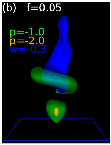
Cases are identified with prefixes of four characters, which is short for historical reasons: it fits within four bytes. For example, aaaa.input configures case {aaaa} with the viscosity (inverse Reynolds number) to be rei=.0004 and the Coriolis parameter f to be swirl=.05. Somewhere within the simulation you should be able to get a snapshot like this, captured with the deprecated vis5d software:

The frequency at which the model dumps all the fields (and time derivatives of fields, so the model can in principle be exactly restarted) are within filetimes.txt.

$ ln -s aaaa.input box.input
$ ./boxn91

This is what you enter at the prompts. It will take the model out to the dump of the dump of ~/boxout/aaaad010000.sav.

[L boxprogram]$ ./boxn91
 continue from previous case?
0
  enter four characters: 'case'
'aaaa'
  Current parameters are:
 &F
 REI     =  3.9999999E-04,
 REIT    =  1.0000000E-03,
 SWIRL   =  5.0000001E-02,
 DTMAX   =  0.1000000    ,
 ALIM    =  0.2000000    ,
 DIFF    =  0.1000000    ,
 PIT     =   3.000000    ,
 RLX     =   1.500000    ,
 GAMMA   =  0.3000000    ,
 SLIP    =   2.000000    ,
 ORDER   =   5.000000    ,
 EX2     =  0.0000000E+00,
 EX3     =  0.0000000E+00,
 EX4     =  0.0000000E+00
 /
  Do you want to change any parameters?
  enter yes, and store=2, yes, no store=1, no=0
0
 dtdif=  2.0603456E-02
 time now =  0.0000000E+00  enter tstop,tdiag
10,.01

After about ten minutes of wall clock, the model should make it out to time=10 (dimensionless).

    4844.    9.980 0.002060   0.67087   0.67087  -0.04251
    4849.    9.990 0.002060   0.67100   0.67100  -0.04268
    4854.   10.001 0.002060   0.67112   0.67112  -0.04284
  FINISHED!
 nloc=        4854   elapsed/nloc  0.0000000E+00  millisecs
 time=   10.00070       cput=  0.0000000E+00  steps=   4854.000   

The numbers you see are also within aaaa.hist, which will be appended to after restart. Here is what the numbers mean:

    4854.   10.001 0.002060   0.67112   0.67112  -0.04284
    step #   time    dt       max speed  max w    min pressure

The numbers are diagnosed for the central part of the domain, and z<.5, roughly the domain portion seen in the above snapshot.

Next we show how to restart the model.

$ rm restart.sav
$ ln -s ../boxout/aaaad010000.sav restart.sav
$ ./boxn91

Here is way it looks for me. Note there is a dump of the vertical profile of viscosity. Apparently I was having some confusion/problem about this at some time, so that is why the dump shows up. Note a the number 20.00000 is spit out, which is the time for the next file dump, as acquired from filetimes.txt.

[L boxprogram]$ ./boxn91
 continue from previous case?
1
           1  0.0000000E+00  3.9999999E-04  3.9999999E-04
           2  4.4620000E-03  3.9999999E-04  3.9999999E-04
           3  9.0290001E-03  3.9999999E-04  3.9999999E-04
           4  1.3805000E-02  3.9999999E-04  3.9999999E-04
           5  1.8893000E-02  3.9999999E-04  3.9999999E-04
           6  2.4390001E-02  3.9999999E-04  3.9999999E-04
           7  3.0393001E-02  3.9999999E-04  3.9999999E-04
           8  3.6991000E-02  3.9999999E-04  3.9999999E-04
           9  4.4270001E-02  3.9999999E-04  3.9999999E-04
          10  5.2308001E-02  3.9999999E-04  3.9999999E-04
          11  6.1175998E-02  3.9999999E-04  3.9999999E-04
          12  7.0941001E-02  3.9999999E-04  3.9999999E-04
          13  8.1660002E-02  3.9999999E-04  3.9999999E-04
          14  9.3382001E-02  3.9999999E-04  3.9999999E-04
          15  0.1061500      3.9999999E-04  3.9999999E-04
          16  0.1200000      3.9999999E-04  3.9999999E-04
          17  0.1349580      3.9999999E-04  3.9999999E-04
          18  0.1510460      3.9999999E-04  3.9999999E-04
          19  0.1682760      3.9999999E-04  3.9999999E-04
          20  0.1866550      3.9999999E-04  3.9999999E-04
          21  0.2061860      3.9999999E-04  3.9999999E-04
          22  0.2268610      3.9999999E-04  3.9999999E-04
          23  0.2486730      3.9999999E-04  3.9999999E-04
          24  0.2716050      3.9999999E-04  3.9999999E-04
          25  0.2956400      3.9999999E-04  3.9999999E-04
          26  0.3207550      3.9999999E-04  3.9999999E-04
          27  0.3469230      3.9999999E-04  3.9999999E-04
          28  0.3741180      3.9999999E-04  3.9999999E-04
          29  0.4023070      3.9999999E-04  3.9999999E-04
          30  0.4314580      3.9999999E-04  3.9999999E-04
          31  0.4615390      3.9999999E-04  3.9999999E-04
          32  0.4925120      3.9999999E-04  3.9999999E-04
          33  0.5243420      3.9999999E-04  3.9999999E-04
          34  0.5569940      3.9999999E-04  3.9999999E-04
          35  0.5904310      3.9999999E-04  3.9999999E-04
          36  0.6246150      3.9999999E-04  3.9999999E-04
          37  0.6595120      3.9999999E-04  3.9999999E-04
          38  0.6950850      3.9999999E-04  3.9999999E-04
          39  0.7313000      4.6260000E-04  4.6260000E-04
          40  0.7681220      5.3624407E-04  5.3624407E-04
          41  0.8055170      6.1103405E-04  6.1103405E-04
          42  0.8434540      6.8690802E-04  6.8690802E-04
          43  0.8819000      7.6380005E-04  7.6380005E-04
          44  0.9208260      8.4165210E-04  8.4165210E-04
          45  0.9602020      9.2040398E-04  9.2040398E-04
          46   1.000000      1.0000000E-03  1.0000000E-03
  continuing with aaaa
   20.00000    
  Current parameters are:
 &F
 REI     =  3.9999999E-04,
 REIT    =  1.0000000E-03,
 SWIRL   =  5.0000001E-02,
 DTMAX   =  0.1000000    ,
 ALIM    =  0.2000000    ,
 DIFF    =  0.1000000    ,
 PIT     =   3.000000    ,
 RLX     =   1.500000    ,
 GAMMA   =  0.3000000    ,
 SLIP    =   2.000000    ,
 ORDER   =   5.000000    ,
 EX2     =  0.0000000E+00,
 EX3     =  0.0000000E+00,
 EX4     =  0.0000000E+00
 /
  Do you want to change any parameters?
  enter yes, and store=2, yes, no store=1, no=0
0
 dtdif=  2.0603456E-02
 time now =   10.00070      enter tstop,tdiag
200,.01

You will need more than 190 minutes for the model to complete. As the tornado spins up, the model reduces the time step to satisfy the CFL condition.

After the model finishes, you should have time series in aaaa.hist that can be plotted.

$ python plothist.py aaaa

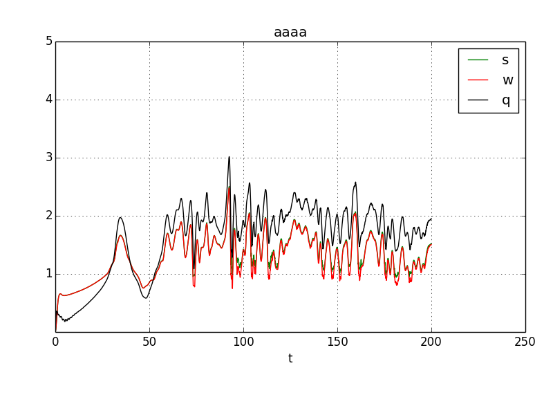
You should see something like this, traces of the maximum values of speed, w and q:

Note q in the plot is a way of plotting pressure as a speed. It is the speed that Bernuolli's equation predicts could be accelerated by the low pressure $q=\sqrt{2|p|}$.

The absolute value just keeps the code from blowing up; the negative values of p are producing the extreme values of q that are plotted.

The python plotting programs for the fields within the .sav files require first converting the .sav files to a pickle file. This one-time conversion makes it very easy to read the data into a variety of python plotting programs. Here we do an example with the final output at time=200.

$ python sav2pkl.py ~/boxout/aaaad020000.sav

To see the grid at the surface and in a vertical cross-section through the center:

$ python gridplot.py ~/boxout/aaaad020000.pkl
$ display grid_xy.svg
$ display grid_xz.svg

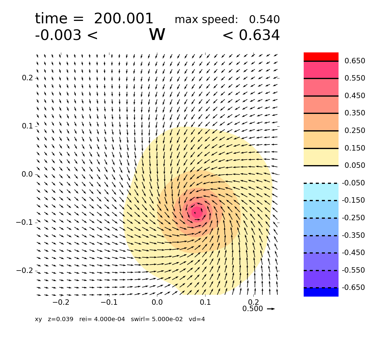
To a see an ugly plot of the vertical velocity at z=.06, together with horizontal wind vector plotted on 1/16th of the grid points, do:

$ python plotpkl.py ~/boxout/aaaad020000.pkl
$ eog w20000.png 

Plots of the fields will be more effective after we focus on the region where the vortex is. The domain is -2<x<2 -2<y<2 and 0<z<1. We make a new .sav file that stores cuts out -.25<x<.25 -.25<y<.25 and 0<z<.5 and interpolates the fields to a Cartesian, isotropic grid.

Currently, cubit is a bit clumsy to run. Here is how we do it:

$ cd ../boxout
$ ~/boxprogram/cubit

You need to enter some text at the query:

[L out_aaaa]$ ~/boxprogram/cubit
  enter 'case' ,num
'aaaa', 200000

Here is the tail end of what I see dumped to the monitor:

 interpolated grid size=  3.9062500E-03
 minimum model grid size=  1.3805000E-02
 aaaad200000.sav  aaaaa200000.sav

Note the fifth character in the original .sav file is d, the altered (interpolated) .sav file has an a. There is no particularly good reason for this designation.

$ cd ~/boxprogram
$ python sav2pkl.py ~/boxout/aaaaa200000.sav
$ python plotpkl.py ~/boxout/aaaaa200000.pkl
$ eog w20000.png 

Here is what I see:

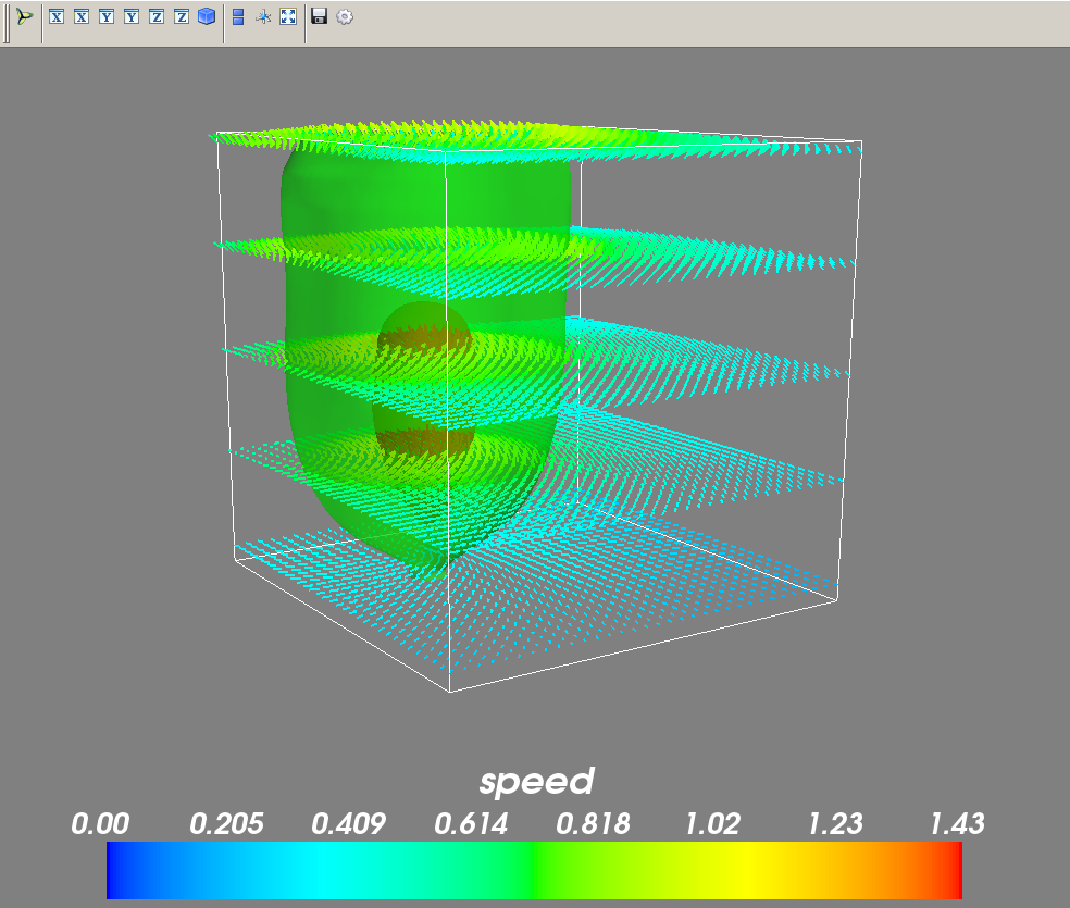
python isovectpkl.py ~/boxout/aaaaa200000.pkl 

A GUI should pop open, showing the p=-1 and p=-.5 isosurfaces. Note the upper left icon allows some features of the rendering to be switched on or off. Dexerity and creativity with a two-button mouse is also essential to change the viewing of the rendering.

Note that it is possible to identify a time period of interest and restart the model from a .sav file, with more dump times specified within filetimes.txt.

It is also possible to double the resolution before restarting.

$ cd ~/boxout
$ ../boxprogram/dubl181

Here is what I did:

[L out_aaaa]$ ../boxprogram/dubl181
  enter 'case' ,num, 'newcase' 
'aaaa',200000,'bbbb'

This makes a new file bbbbE200000.sav.. By the way, the E does not mean much anything special … maybe Extended? In order to start from this file, you need to edit box.size to be

c       PARAMETER(In=361,Jn=361,kn=181,
c       PARAMETER(In=91,Jn=91,kn=46,
        PARAMETER(In=181,Jn=181,kn=91,
     &            im=In-1,Jm=Jn-1,km=kn-1)

and then compile again

$ ifort -o boxn181 boxn.f boxs.f

Proceed with your computations using boxn181

What isn't shown in this tutorial is how to make animations, such as seen here: http://mensch.org/suction/

box (last edited 2014-06-17 10:24:43 by BrianFiedler)