Radiative Convective Equilibrium
Contents
This page describes a series of simulations with a radiative convective model (RCM), run out to radiative convective equilibrium. The RCM is based on the CRM radiation code, that has been offered online for almost a decade. (The model results shown here are based on the revised code, as described at that site). The RCM is written in Python. The RCM code uses Python's subprocess module to send the input file and retrieve the output file, without actually writing it to disk. Python's text handling abilities are well suited for constructing the text input files and then parsing through the output file to find the heating rates that are used to update the temperature. Typically, the RCM calls the CRM 2000 times, and updates the temperatures with a half-day time step.
The RCM model extrapolates the temperature profile, which is from the mid-points of the levels, to a surface air temperature. (Oddly, the surface air temperature in the CRM input file is not actually used by the CRM. The skin temperature is what is actually important and is used by the CRM.) The surface air temperature is then used to calculate the sensible heat flux as:
SENSFLUX = SENSFLUXCOEF*(TSKIN-TSURAIR)
where the default value for SENSFLUXCOEF is 20 W m-2 K-1.
When water vapor is allowed to adjust, it adjusts to keep the relative humidity at 68% times pressure/(surface pressure). Except, where temperature has begun to increase with height, the specific humidity from the lowest temperature layer is retained. (This is the so-called tropopause cold trap). Optionally, specific humidity can be retained from a previous model run, and required to remain invariant in time.
Model labels:
stn, standard lapse rate of 6.5 K km-1 is used for the convective adjustment
mst, moist adiabatic lapse rate is used for the convective adjustment
rad, no convective adjustment, and no sensible heat flux from the surface
2x, CO2 is doubled from 355 ppmv to 710 ppmv
w, specific humidity if being held constant, from a previous model run
sol, downward solar radiation at the top of the atmosphere increased by 5%
Standard
model label: stn
- Convective adjustment with the standard lapse rate.
Note: the final input file to the CRM, and thus one consistent with radiative convective equilibrium, is offered at CRM Online as radconeq.in. For your information, that file is also here, but with the temperature replaced by a *, because those numbers are continually updated by the model.
|
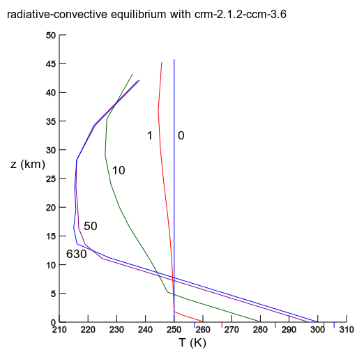
stn: Initialized at 250 K and run out to 630 days. The day is indicated on the profile. The time-step is less than or equal to 0.5 days (less at beginning and end). The tick marks on the T axis are the skin temperature. |
|
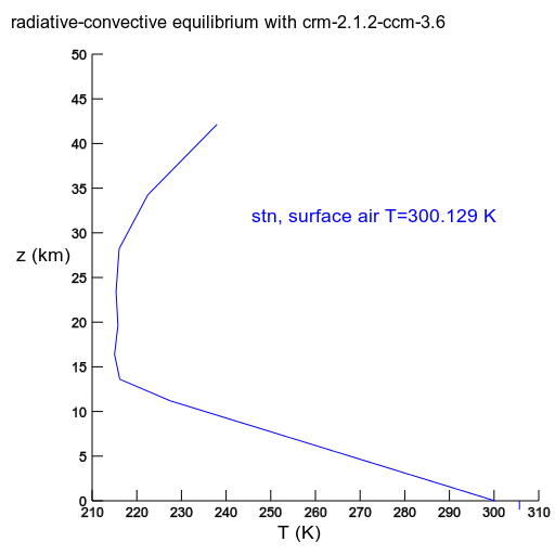
stn: The equilibrium profile profile at 630 days. Final flux balance at the top of the atmosphere is within 0.1 W m-2. The downward blue tick mark at 305.7 K denotes the skin temperature. |
|
|
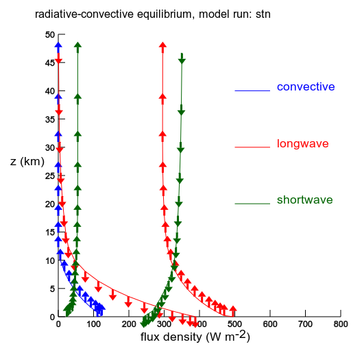
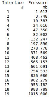
Vertical flux densities for the equilibrium stn simulation. The lowest blue arrow is the sensible heat flux from the surface. The blue arrows above that are the exchange fluxes in the convective adjustment. The pressure levels of the flux density calculations are listed. They remain constant throughout the model run. |
|
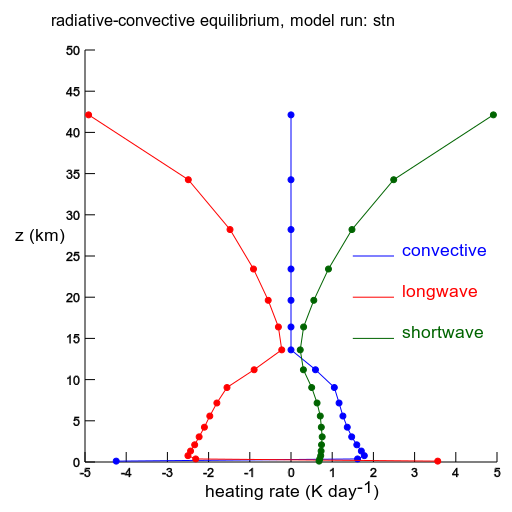
Heating rates for the equilibrium stn simulation. Note that infrared radiation generally cools the atmosphere, but adjacent to lower boundary, the infrared radiation is heating the atmosphere. This is because of the relatively large temperature difference between the ground and the air immediately above it. As a consequence, there must be a large convective heat flux out of the lowest layer of air, and thus cooling by the convective heat flux. |
Double CO2
model label stn2xw: with specific humidity retained (from stn)
model label stn2x: with relative humidity specified (specific humidity adjusting)
|
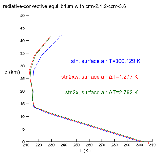
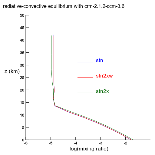
stn2x and stn2xw are equilibrium solutions with double CO2, but otherwise the same parameters as stn. stn2xw has specific humidity identical to stn. stn2x has the relative humidity identical to stn, except possibly in the stratosphere, where the "cold trap" at the tropopause may enforce a slightly different relative humidity. |
|
The mixing ratio. Notice the red curve overlies the blue. |
Turn off convection
|
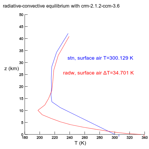
radw has specific humidity retained from stn. The convective adjustment and the sensible heat flux from the surface is turned off. |
|
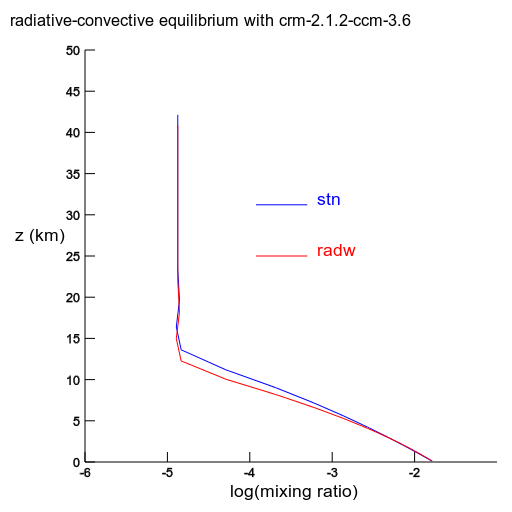
Specific humidity is invariant. If plotted with respect to pressure levels, these curves would overlap. But, being plotted with respect to z levels, they don't. |
Moist adiabatic adjustment
|
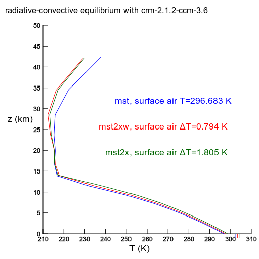
As in the stn simulations, but using the moist adiabatic lapse rate. The moist adiabatic lapse rate decreases as temperature increases. This property leads to a negative feedback in global warming forced by radiation. The specific comparison demonstrating the negative feedback is to compare the ΔT in mst2x with stn2x. |
|
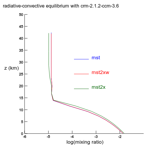
The mixing ratio. Notice the red overlies the blue. |
Increase solar radiation
|
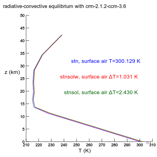
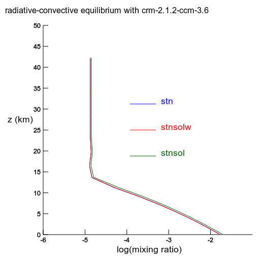
Warming forced by changing the solar constant in the model from 700 W m-2 to 710 W m-2. The model has fixed zenith angle, with cosine=0.5. So the change in incoming solar radiation is 5 W m-2. Being cloudless, the model has an albedo of approximately 0.16. So the radiative forcing at the top of the atmosphere is 4.2 W m-2, comparable to double CO,2. |
|
The mixing ratio. |
